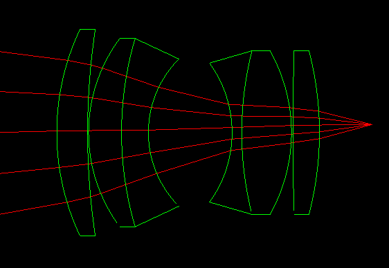
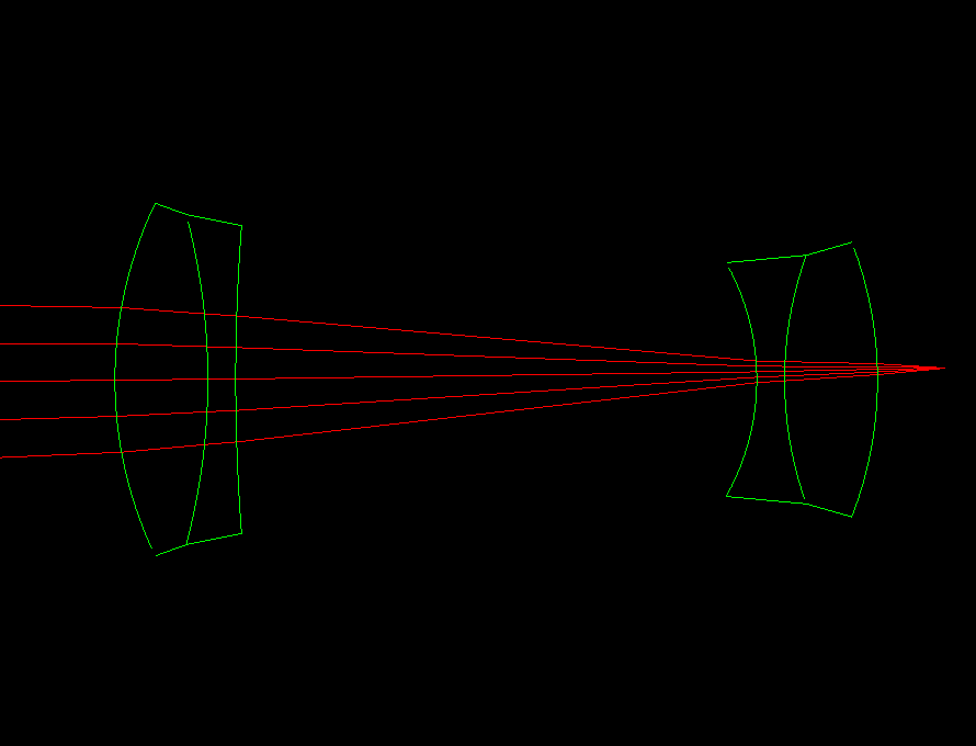
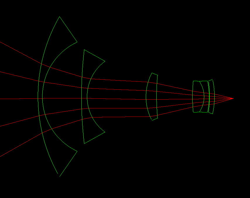
Lens shape (lenstester demo)
|
|
|
|
|
|
|
|
|
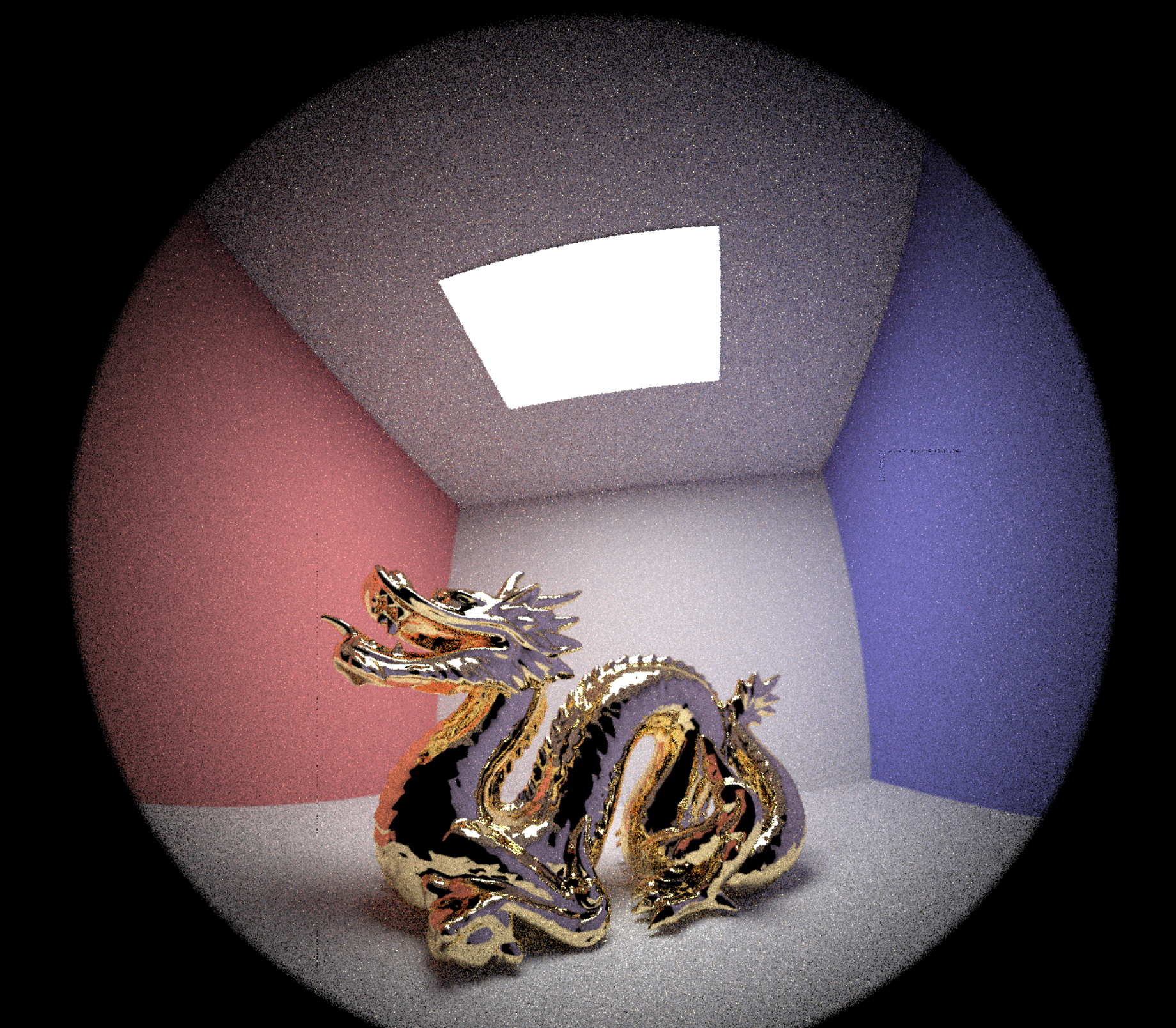
Our project, Pathtracing Lenses and Autofocus, is a project which simulates raytracing through real camera lenses to achieve realistic effects on rendered scenes. This includes ray refraction through lenses, rendered image modification due to differing focal lengths and compound lens structures, and varying sensor depth to alter the plane of focus. We also implemented various autofocus algorithms which support automatic setting of the sensor’s depth to bring a desired object into focus. The autofocus is performed based on searching for the best sensor depth based on evaluating a focus metric on a patch the user can select which contains the desired object. We implemented various focus metrics for this process to experiment with the consistency and quality of the autofocus. Additionally, we added changes to improve the speed of the autofocus, through a new search algorithm as well as modification of the pathtracer’s parameters when performing the autofocus. Our newly introduced focus metrics performed well in producing highly-focused images across the board with reasonable patch selection, and using our modified focus-depth search algorithm alongside decreasing the path-tracer’s parameters when performing autofocus both increased the speed of the autofocus significantly. Our project also includes a GUI which allows users to experiment with different pathtracer parameters, focus metrics, and search algorithms with rendering and autofocusing on various scenes.
Following the Spring 2016 project spec for Lens Simulator, we first tried to get our PathTracer project code working with the new Lens Simulator code. This was actually much harder than anticipated. None of us were able to get the 2016 Lens Simulator code to compile on our systems, so we first tried to migrate over the important files from the 2016 version (lenscamera, lenstester) and integrate them with our current PathTracer. However, we ran into many issues because the current PathTracer project is set up differently than the 2016 PathTracer (for example, the split of the old pathtracer.cpp from 2016 into raytraced_renderer.cpp and pathtracer.cpp). This led to us getting numerous issues like recursive header dependencies which we weren’t able to fix. In the end, we decided to instead start with the 2016 version, and try to fix the build issues and migrate our PathTracer code.
Fixing the build errors required us to modify the CMakeLists.txt files and update the outdated CGL with our new one. This required extensive updating of the code, for example, updating all uses of Spectrum to Vector3D. We also had some problems building on Mac systems, but were eventually able to fix this. With a working base Lens Simulator project that compiled on all our systems, we were finally able to start working and implement raytracing through lenses and a contrast-based autofocus as described in the project spec. Our contrast-based autofocus works through a variance-based focus metric, which is a function that takes in an image, and returns a value that denotes how “in focus” the image was. So, our autofocus just linearly scans through potential sensor depths, renders the image, and uses the focus metric to find the depth that was most in focus.
Autofocus Search MethodsWith the project spec completed, we finished working on most of the planned deliverables in our proposal. Next, we decided to work on speeding up the autofocus mechanism. As hinted in the project spec, we wanted to use the fact that the focus improves as we approach the correct image depth, and then degrade as we move away. To exploit this, we made a simple divide and conquer peak finding algorithm to find the correct sensor depth. To find the peak in a range, we take the midpoint of the range and evaluate the focus metric at that point. Then, we take one step_size step to the left and right, and evaluate the focus metric at those points. Then, we either return the midpoint if it was higher than the left and right, or recurse down into either the left or right sections depending on the evaluation. However, this implementation was not very good, as there was a lot of noise in the results. To fix this, we ended up evaluating two points on the left and two on the right (so along with the middle point, five), and then comparing the mid value to the max of the two left or two right. This ended up with much better results, usually giving us a good focus depth in a fraction of the time.
Our final search method “Combined”, works as a multi-phase linear search with adaptive step size and search range, followed by a fitting of points to a polynomial. First, we find a base-line peak-depth using linear search, which is repeated in a new search area and new step size multiple times based on the depth found in the current search, until the peak found by the search only changes by a sufficiently low amount (convergence). Then, we sample several points near this peak depth and push these samples (9 pairs of sensor-depth to metric values, 9 is small for speed while being large enough to form a well-defined quadratic shape, based on experiments) into a vector. Finally, we perform quadratic regression to fit the samples to a curve, and select the sensor depth at the peak of this curve as the final sensor depth. While this did not perform exceptionally better than the other methods, it is more precise, and the lack of a gap is likely due to the fact that the linear and DAC algorithms already produce very good results.
Autofocus ParamsIn addition, we changed the original bump settings for auto-focusing from -s 16 -m 16 -l 5 to -s 8 -l 4 -m 2. This was done to speed up generating images for our data collection process. Downgrading the settings works in this case because the auto-focus procedure doesn’t need high quality images to perform well. This idea is similar to the one in project 3-1 where including two bounces of light already produces a relatively realistic image.
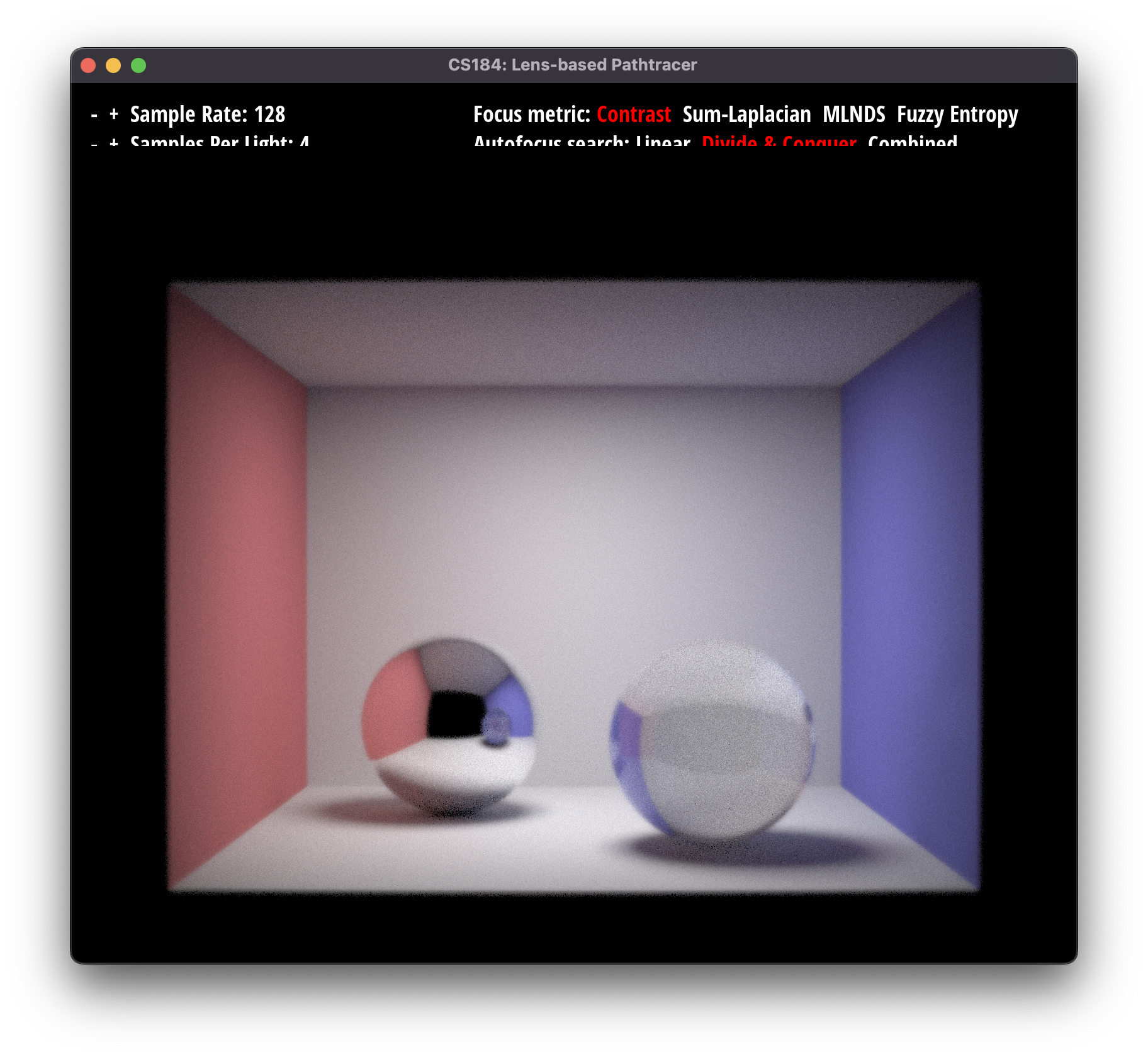
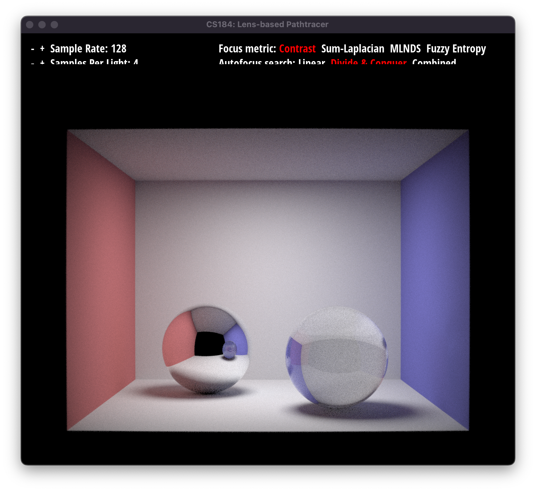
Focus MetricsAs suggested in the Lens Simulator spec, we first tried the Sum-Modified Laplacian metric from the paper Shape from Focus System. First, the RGB values for each pixel were converted to appropriate grayscale values. The grayscale value was calculated as the average of the RGB values. Then, the Laplacian filter was applied along the x and y coordinates. The sum-modified Laplaican value for the pixel located at point x, y is calculated as follows: $f(x, y) = |2 * I(x, y) - I(x - step, y) - I(x + step, y)| + |2 * I(x, y) - I(x, y - step) - I(x, y + step)|$. In our case, we used a step-size of 1. To calculate $\phi$, we used a 3 by 3 window and filtered out the values which were less than our threshold $T_1 = 1.0$. This metric ended up being the best out of the ones we implemented.
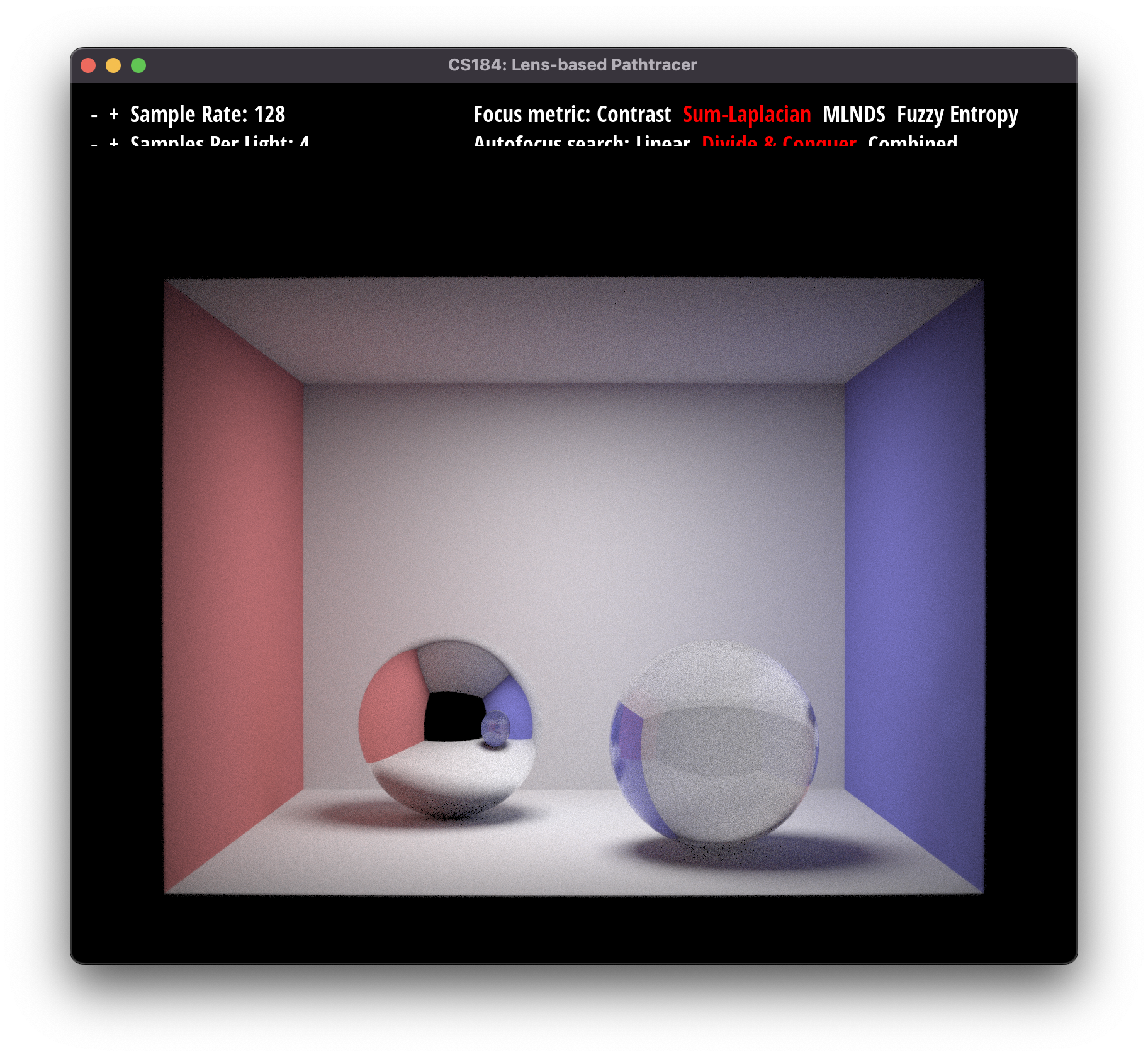
The performance of the Sum-Modified Laplacian metric was very good, but we wanted to see if other metrics could be better. In another paper we found, Learning to Autofocus, the authors described a number of different focus metrics. Out of them, we chose to implement the Mean Local Norm-Dist-Sq metric. This metric is part of a family of metrics that calculate a local measure of contrast by using a gaussian blur. By applying this blur, a local average of colors is created at each point, and then we use this local average to compute the focus metric. First, we create a 2D vector of doubles with a size equal to the dimension of our image, to hold the gaussian kernel. Then, we compute the kernel values according to the following formula: $$G(x,y) = \frac{1}{2\pi\sigma^2}e^{-\frac{x^2+y^2}{2\sigma^2}}$$ For our implementation, we chose $\sigma = 4$ to match the authors. Then, we normalize the kernel. Next, we clone our image, then blur it by convolving the kernel with our cloned image to create our blurred image. Finally, we calculate the metric according to the following formula: $$\phi = \frac{1}{n} \sigma_{x,y} \frac{(I[x,y]-blur(I, \sigma)[x,y])^2}{blur(I,\sigma)[x,y]^2 + 1}$$ where $I[x,y]$ is the intensity of the image at $(x, y)$, and $blur(I, sigma)[x, y]$, is the intensity of our blurred image at $(x,y)$. Finally, to get this metric to match with our search algorithms, we invert the result. This metric was better than the variance metric, but performed slightly worse than Sum-Modified Laplacian and Fuzzy Entropy.
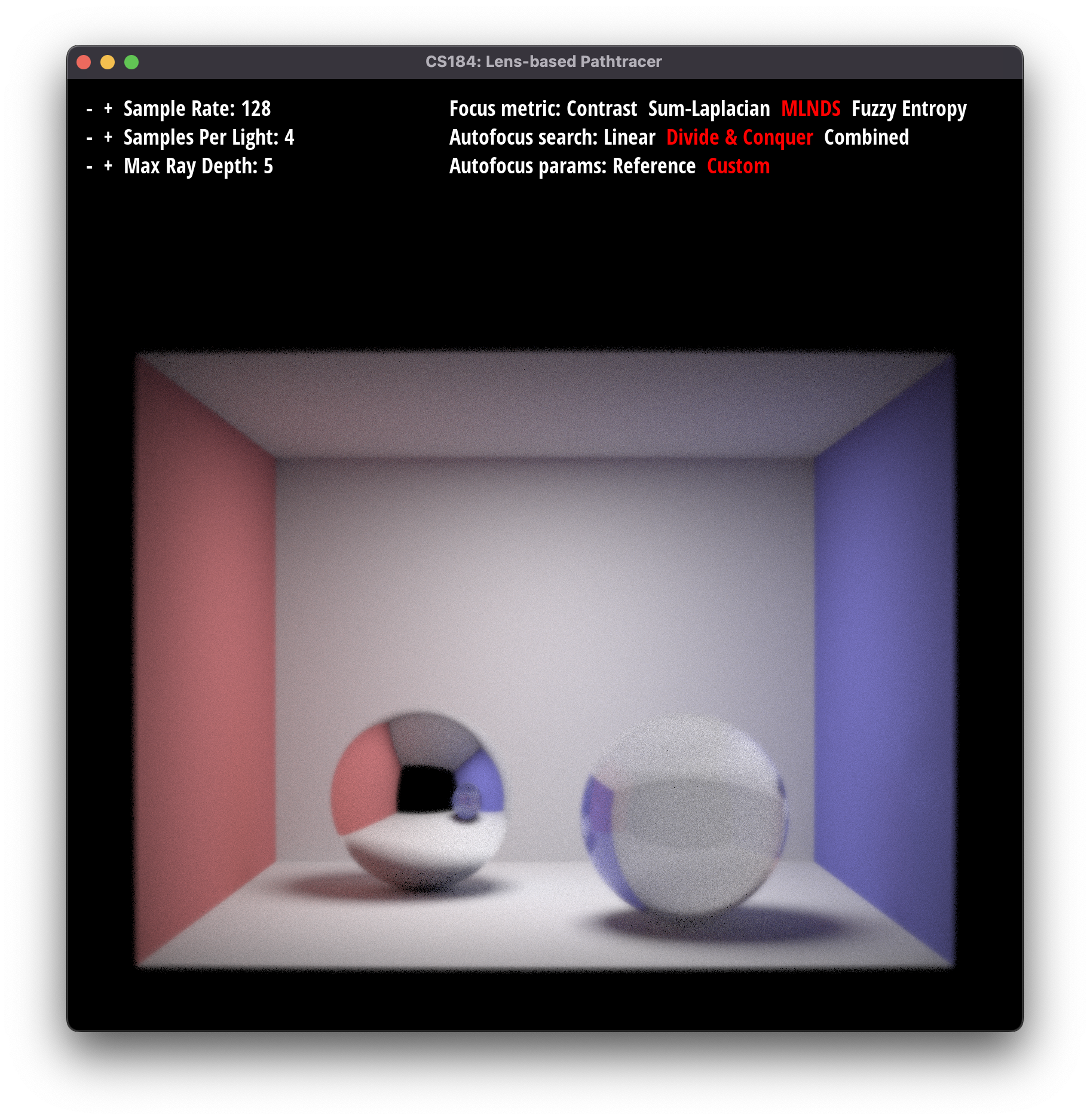
Finally, we decided to implement one more metric, called Fuzzy Entropy, which we found from a paper called An image auto-focusing algorithm for industrial image measurement. First, we create an array of doubles the size of our image to hold our entropy values. Then, for each pixel, we calculate its grayscale value based on its luminosity. We use the following formula: $$C_{greyscale} = 3C_r + 0.59C_g + 0.11C_b$$ With the gray level of each pixel, we calculate $\mu_k$, the membership function of the image fuzzy set with the formula: $${\mu}_k\left(f\left(i,j\right)\right)=\frac{1}{1+\left|f\left(i,j\right)-k\right|}$$ For our implementation, we chose $k = 0.5$. Then, we calculate the fuzzy entropy of this pixel $E_k = -\mu_k \cdot \log(\mu_k)$ and store this in our array. Finally, we calculate the image contrast evaluation for a pixel by looking at its neighboring window of size $w \times w$ pixels (in our implementation, we chose $w=5$). We do this following the formula: $$ {m}_k\left(i,j\right)=\frac{1}{w\times w}{\displaystyle {\sum}_{m=-\left(w-1\right)/2}^{\left(w-1\right)/2}{\displaystyle {\sum}_{n=-\left(w-1/2\right)}^{\left(w-1\right)/2}{E}_k\left(\mu {}_k\left(f\left(i+m,\kern0.5em j+n\right)\right)\right)}} $$ Finally, summing these values in the image contrast map and normalizing them, we get our final focus metric. This ended up performing quite well, usually as good as Sum-Modified Laplacian.
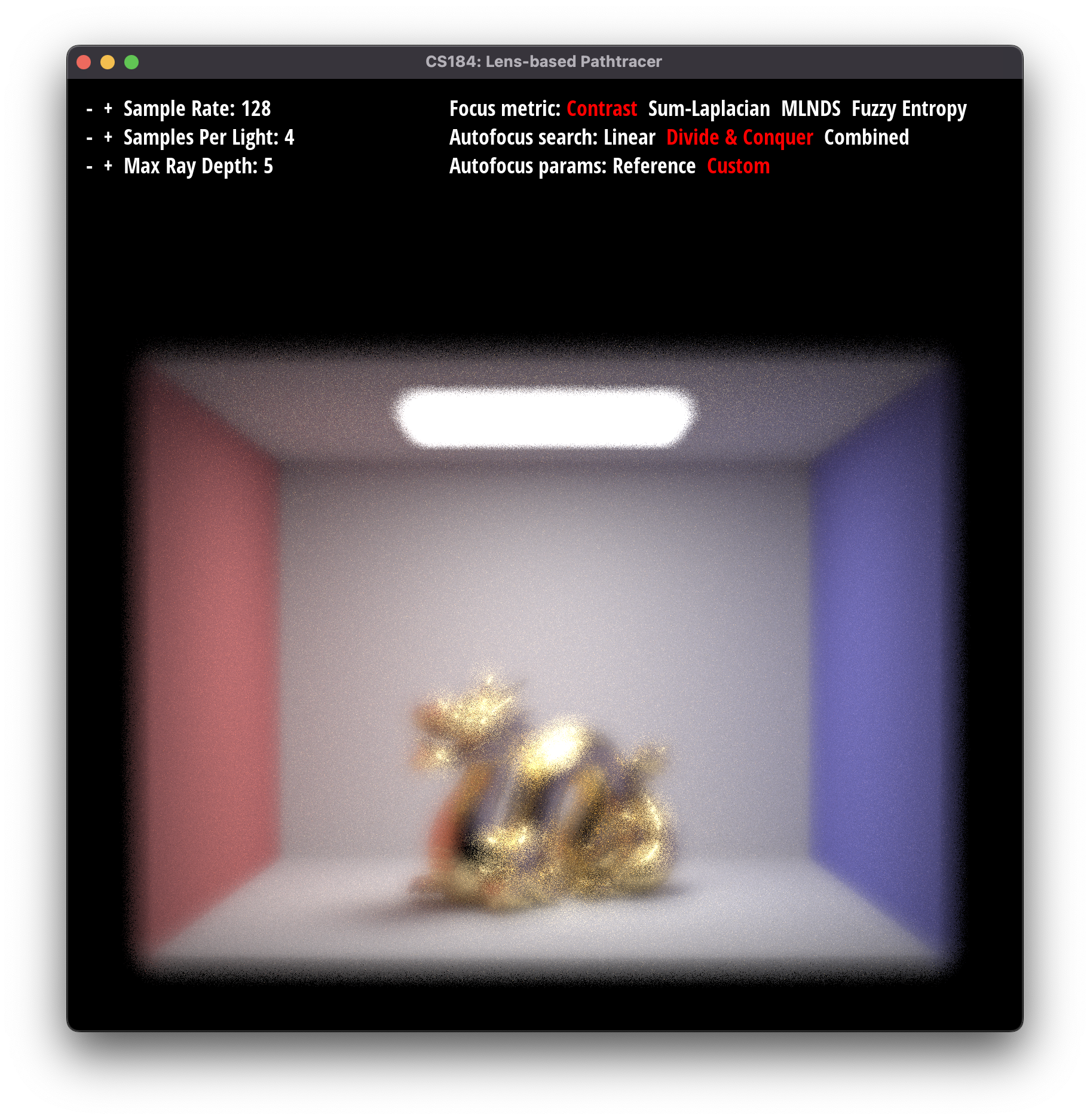
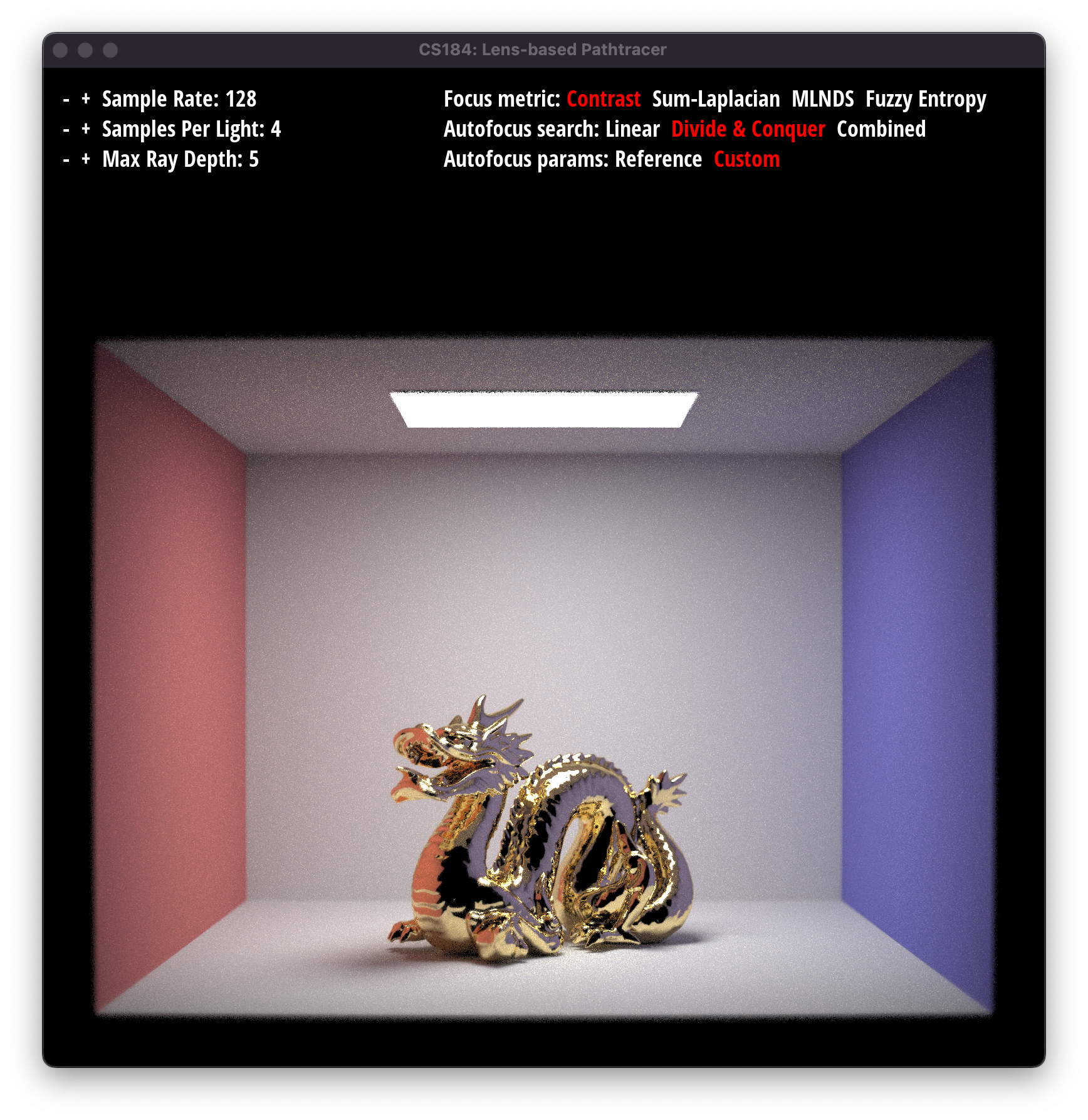
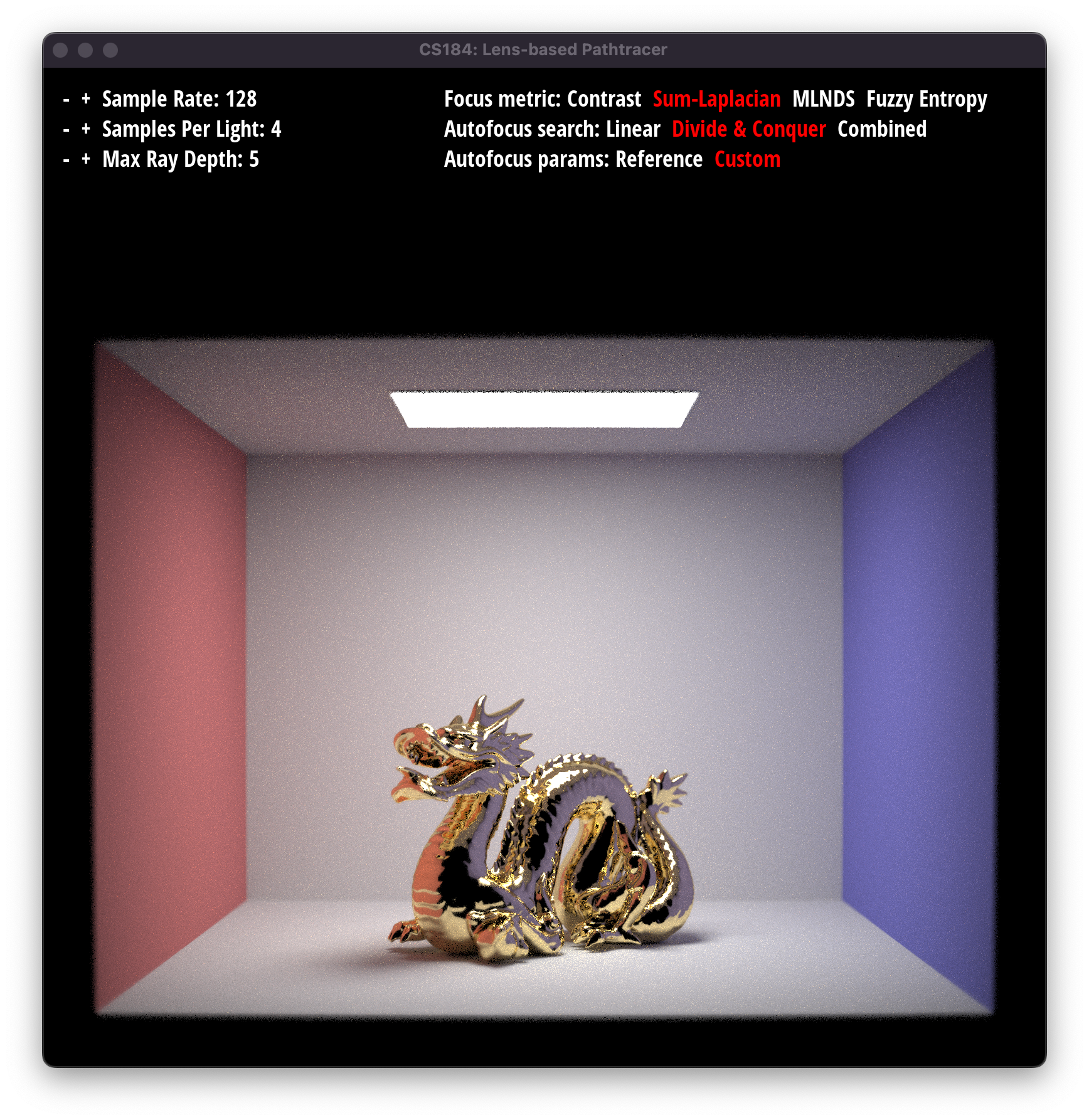
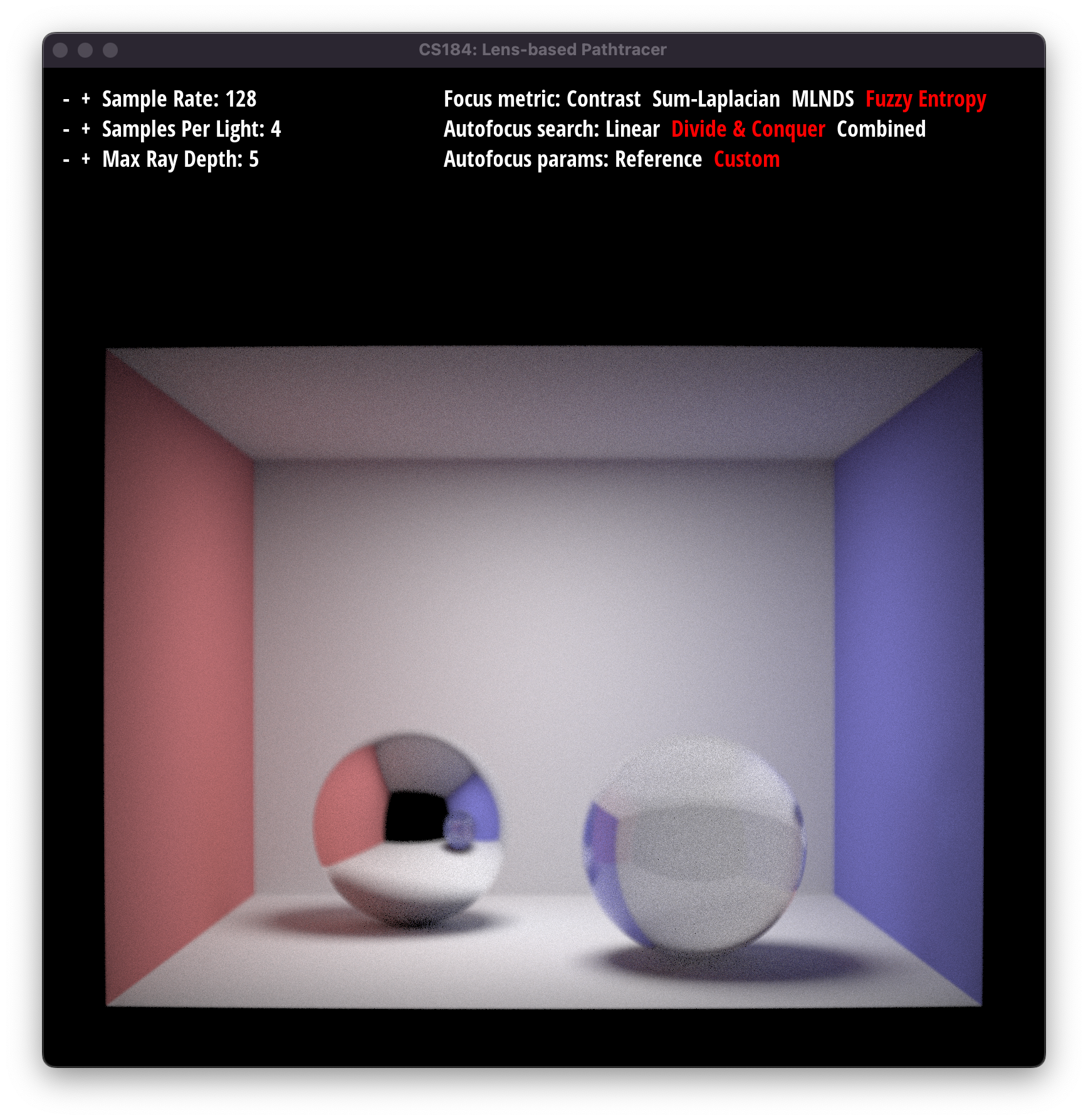
Extra FeaturesWith all these different metrics and search algorithms, we wanted to create an easy method to switch between them as well as change other parameters. To do this, we implemented a GUI at the top of the UI in render mode that would allow you to click to change options. This was also more complicated than expected. We first tried to use the built-in draw_string methods to draw before or after the pathtracer updates the screen, but the pathtracer’s frameBuffer always ended up drawing over our text. To fix this, we created a new variable called ui_height_offset, which marked a size, in pixels, to leave blank at the top of the screen. To implement this, we had to use the OpenGL function glWindowPos2i to change the position that the pathtracer’s frameBuffer would be drawn to. Then, we had to fix the cell rendering mode, as everything was now shifted. This required us to add the ui_height_offset to the coordinates of the cell so it would select the region under our mouse, change the OpenGL code drawing the rectangle so it would appear under our mouse, and fix many other issues like causing crashing when you tried to move the cell selection to this blank region. Once this was done, we now had a blank space at the top of the render mode screen to add custom elements. Then, we added some code to the rendering of text to allow multiple colors in one string (so we could color the selected option red). Finally, we added custom code to mouse_pressed to hook mouse clicks. If the mouse is clicked, we find the position of the click. If it was over any of the pressable text options, we trigger the change.
Finally, the last feature we worked on was automatic autofocus patch selection. This is a relatively simple feature which simply takes a cell selection, presumably a large one with the object of interest in it,renders it with lowered settings if it’s not rendered already, and scans across it in patches of a fixed, small size. At each patch, edge extraction is performed via a 3x3 Laplacian edge detector kernel across the patch, and at the end, the patch with the highest sum of convolved values (theoretically the patch with the most well-defined edge parts, which should follow some boundary along the object of interest) is chosen as the patch for autofocus. This algorithm performed well enough such that we omitted other steps that other algorithms for edge detection typically use, such as first applying a Gaussian smoothing kernel across each patch.
Major Problems EncounteredOne major problem we had to deal with was the issue of memory corruption. After getting the code to compile on all our systems, the code wasn’t completely bug-free. Even though our BSDF code worked in our new PathTracer projects, for some reason the reflections and refractions were incorrect. In addition, for some reason we could not render directly to a file, but using the UI worked. After many hours, we eventually figured out that when rendering directly to a file, for some reason, the c2w (camera to world space) matrix was different from when using the UI directly. We then investigated why this was the case, but found out that none of the the places directly assigning to the c2w matrix were incorrect. Eventually, we narrowed it down to the lines updating the camera’s hFov and vFov. For some reason, the camera’s hFov and vFov vectors were directly on top of the c2w matrix in memory. So, whenever resize was called, the c2w matrix was corrupted, which is why rendering to a file didn’t work. We patched the issue by adding some unused padding bytes to the Matrix3x3 class, which fixed rendering to a file as well as our BSDFs. There were other issues similar to this discovered, for example, there were cases in the code where uninitialized variables were used, which caused many inconsistencies in our program.
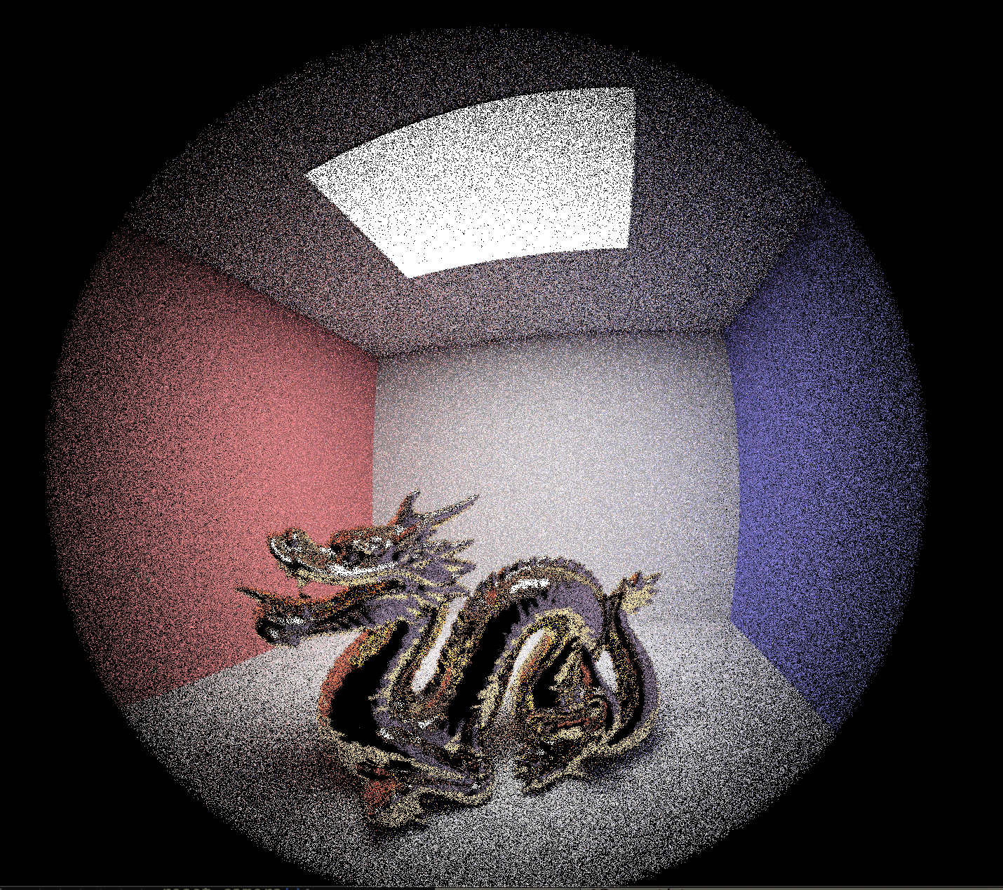
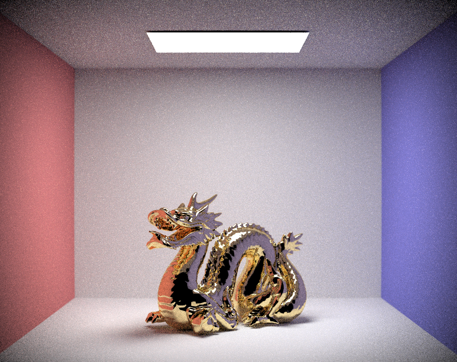
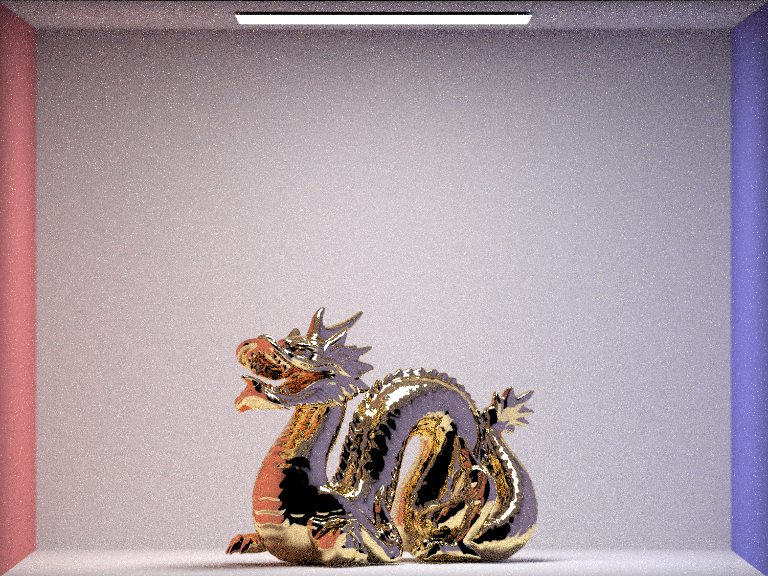
Final lessons we learned:By using lenses with different focal lengths, pathtracer can capture anywhere between a narrow and a wide scene. We tested out autofocus on three distinct lenses with focal lengths of 50mm, 250mm, and 10mm, and it was able to find the best focus for each of them.
Note: There were 4 provided lens settings but only 3 are shown here because two of them provide similar enough result that we decided to omit one.
|
|
|
|
|
|
|
|
|
|
|
|
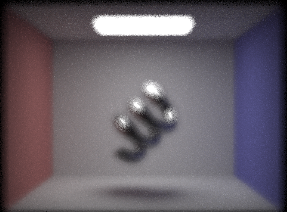
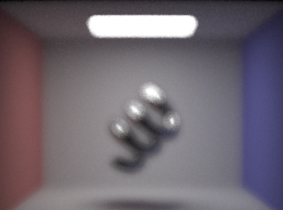
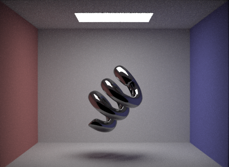
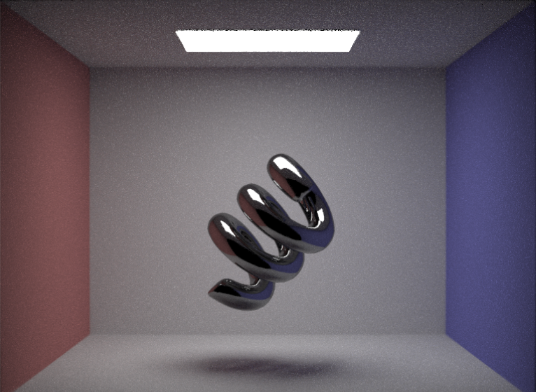
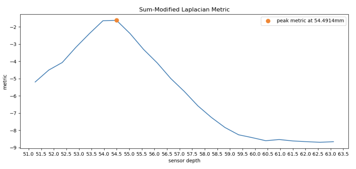
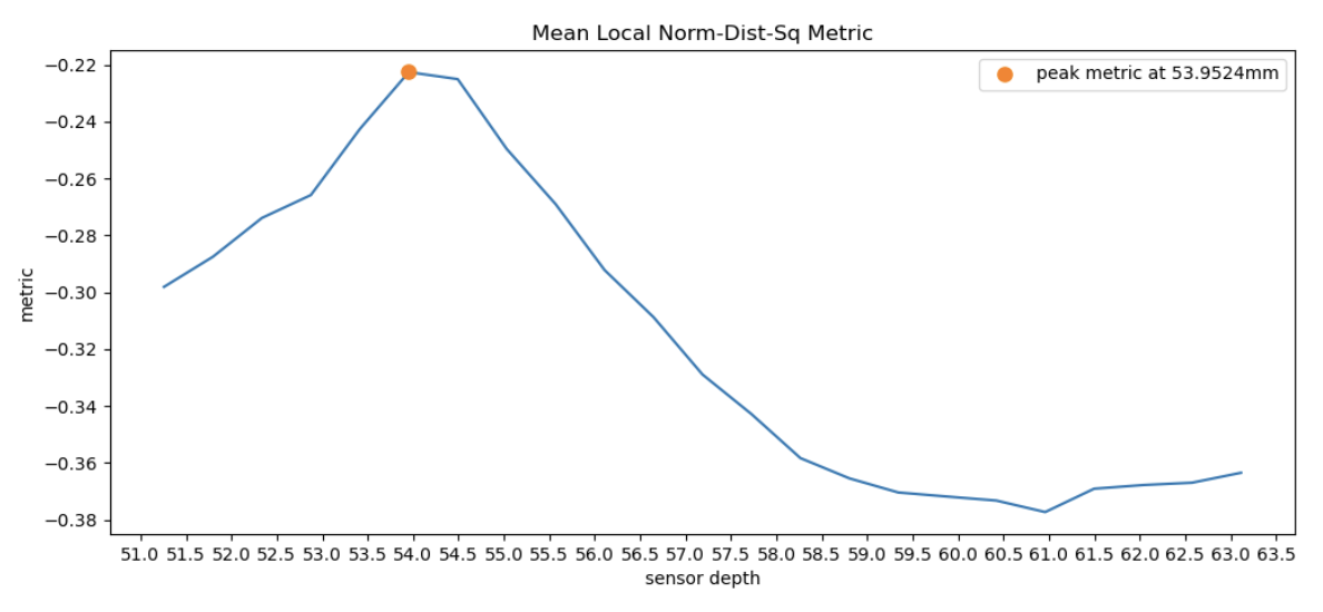
We tried using different focus-evaluating metrics on different dae models and here are the results.
|
|
|
|
|
|
|
|
|
|
|
|
|
|
|
|
|

|
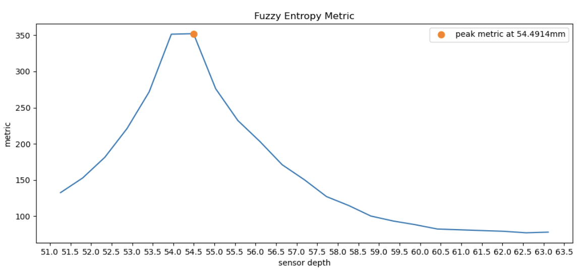
Following from the previous section where we tested different metrics on CBcoil, we observed that variance focus metric failed to find the best sensor depth. To visualize why this is better, we plotted Metrics vs. Sensor depth in graphs for each metric. We can see that all metrics except variance peaked around the correct optimal sensor depth (~54mm), whereas variance is the outlier peaking at 58.8mm.

|
|
|
|
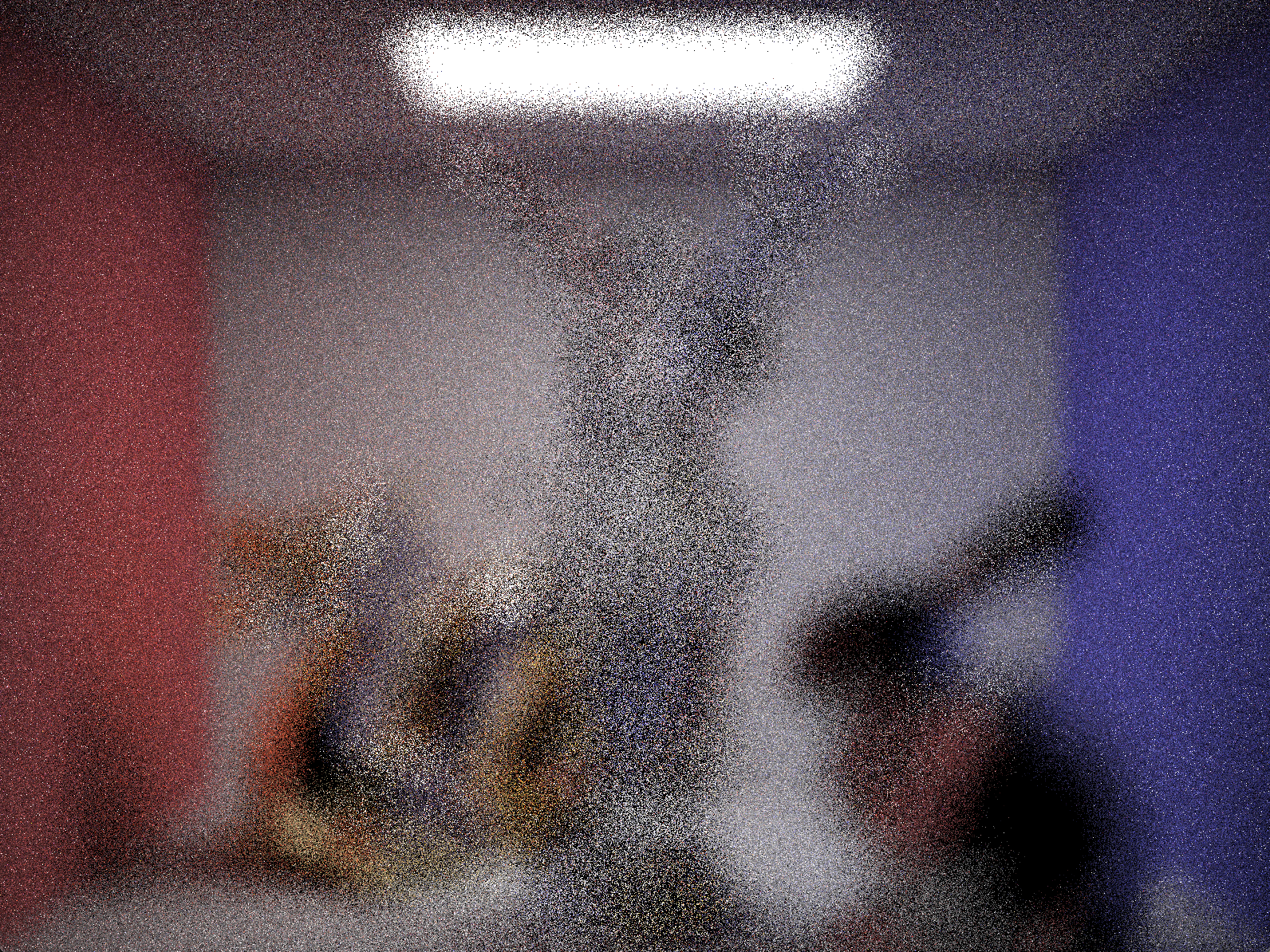
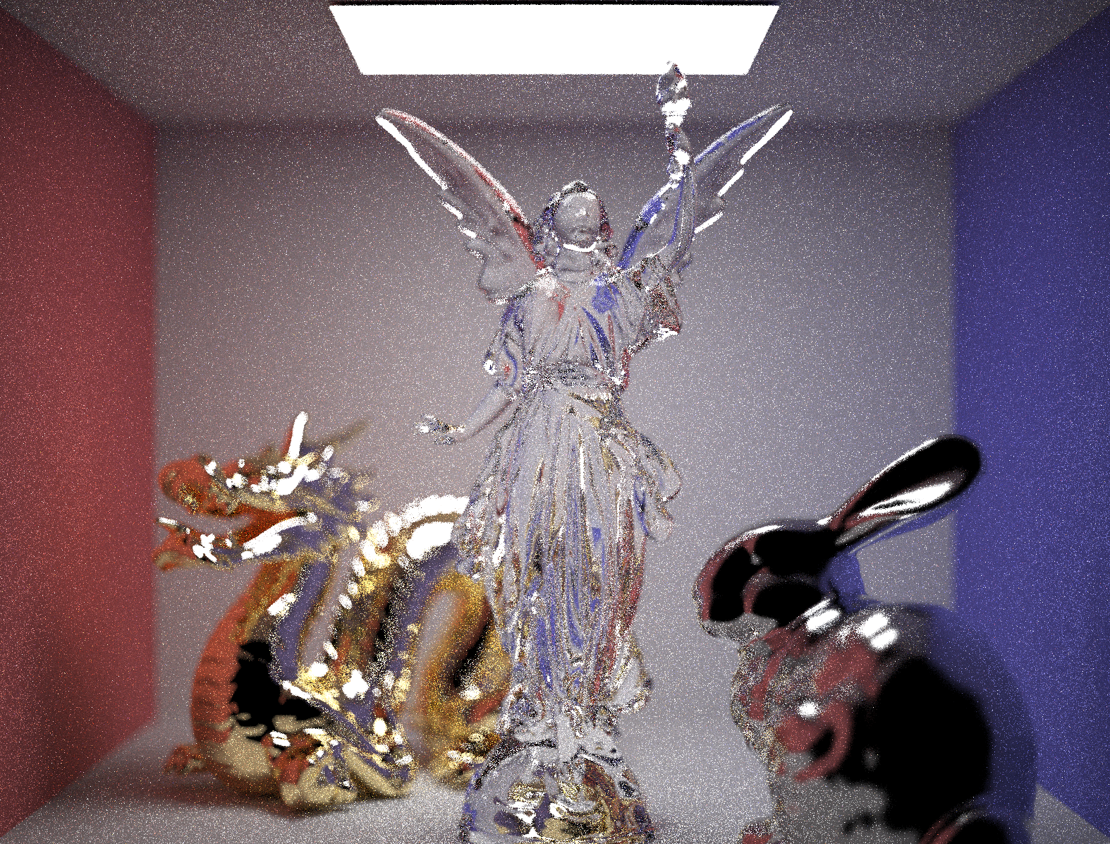
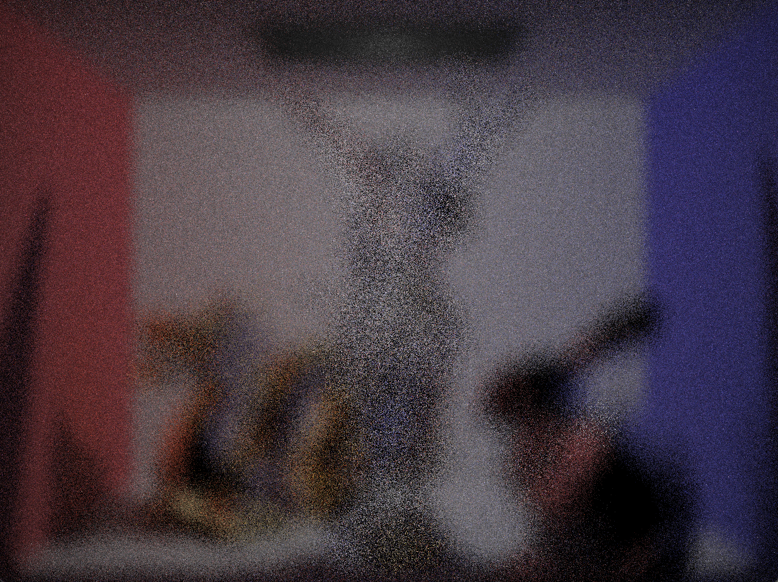
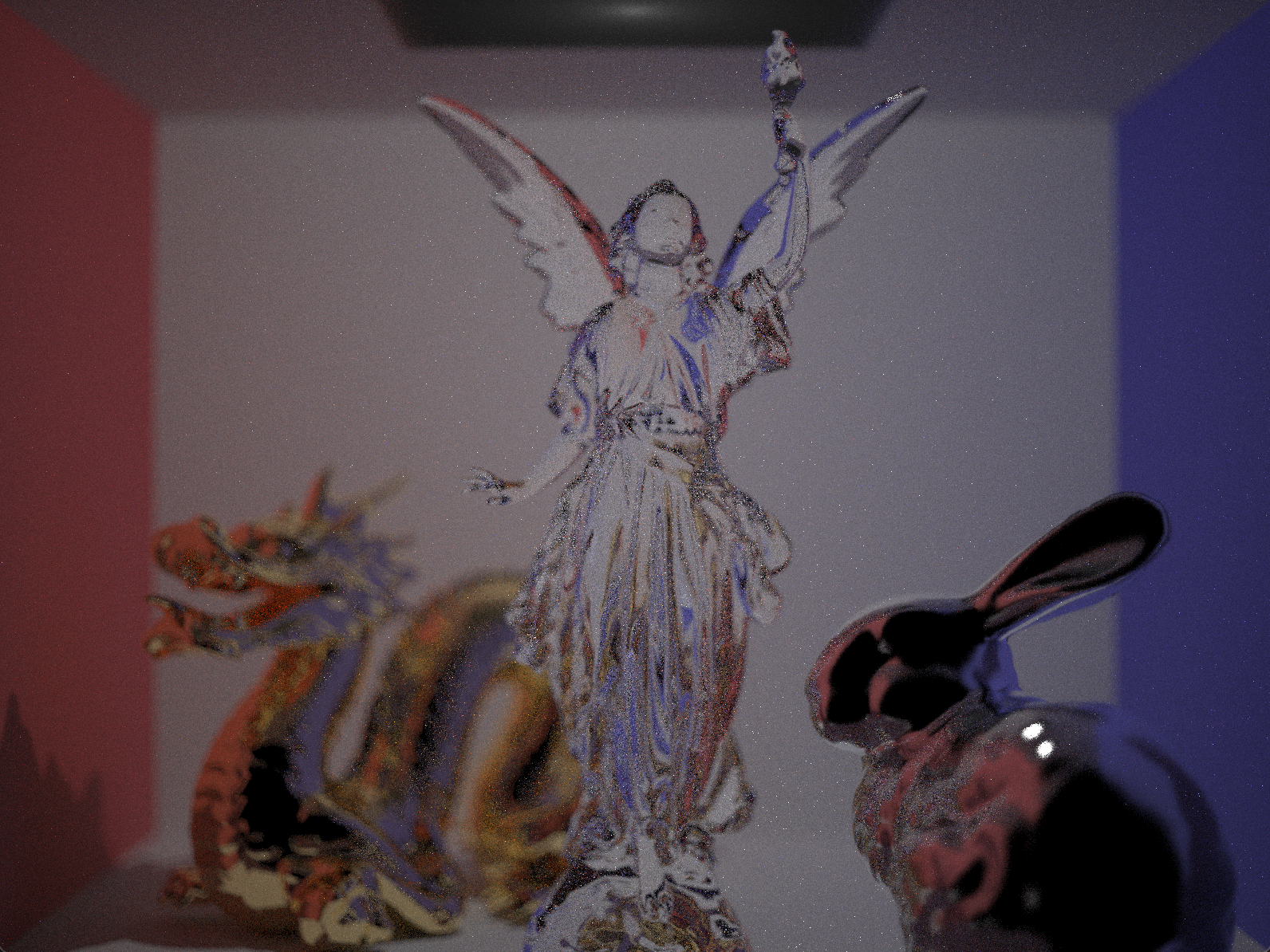
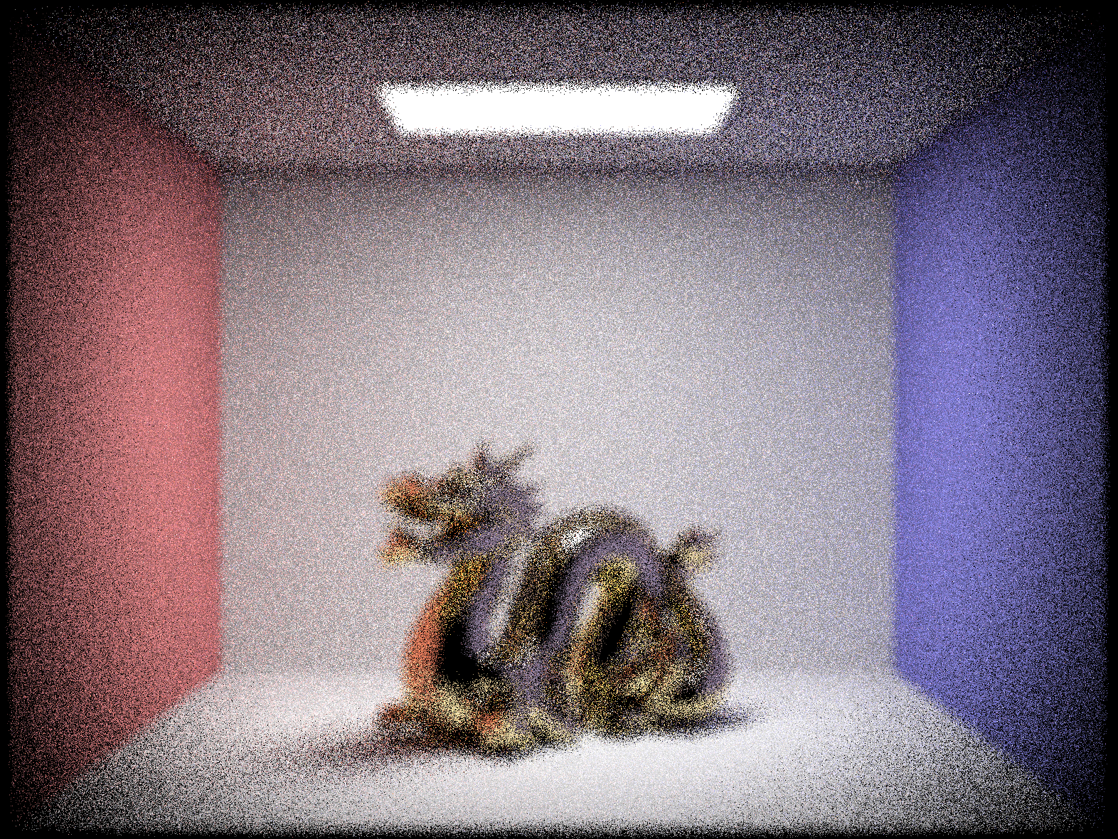
We created a complex scene with three of the demo models together in Blender. We gave each of them different materials. The angel is of glass material, the dragon is a mirror material, and the rabbit is a microfacet material. We also played with light settings and created a bright and dim variation to see how autofocus would react to it. The results show that autofocus was able to find a best focus for the scene in both lighting conditions; however, the image has more noise for the bright scene.